
If you are a regular user of Excel is pretty likely at some stage when you have entered some numbers and Excel that you have seen the cells displaying #### instead of the number that you put into the cell. So why does that happen and how can you fix it?
When #### appears in an Excel cell it means that you have entered a number into the cell in which the column is too narrow to display the number. As a result of this Excel will display #### instead. However, it is important to note that even though the display does not represent the number that you have entered into the cell visually it will still complete any calculations associated with that cell.
This occurs because it is not an error but simply an indication from the program that there is not enough space to display the number entered into the cell accurately. The other thing that excel will do is if it is a very large number it will reduce the size of the number displayed by converting it to scientific form.
For those unfamiliar with the scientific form, here is an example. A cell may contain the number 123,123,123,123. Excel will reduce this number to 1.23 x 10^11. An example of how this is displayed is shown below,

So what can you do to prevent this from happening, particularly in cases where the numbers are very large?
How To Prevent #### From Appearing In A Cell
There are several different strategies you can use to stop #### from appearing in your spreadsheet.
1. Widen The Column
The first and most obvious option is to widen the cell. The easiest way to minimize the width of the cell required is to display the number can be done by double-clicking on the right edge of the column.

2. Reformat The Numbers Into 000’s
The second option for large numbers is to reformat the cells to show the values in thousands rather than the full number. This formatting is generally most appropriate when you are dealing with sales reports where the numbers are normally relatively high.
To do this follow the following steps;
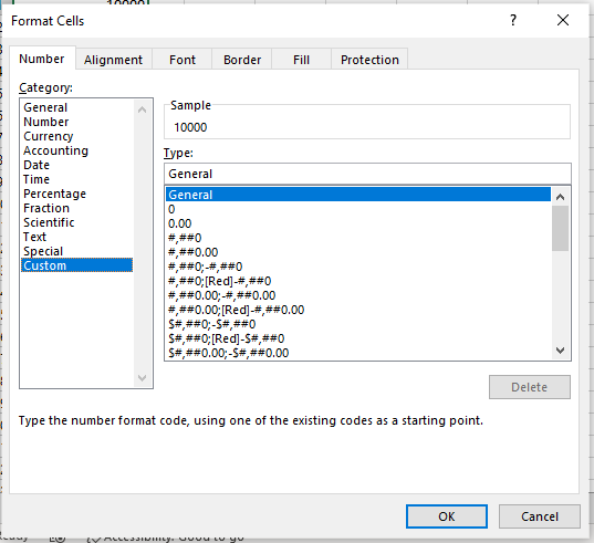
Step 1: Right-click on the cell or if the whole column needs to be formatted right click on the column letter.
Step 2: Select Format Cells

Step 3: Select Custom and #,##0
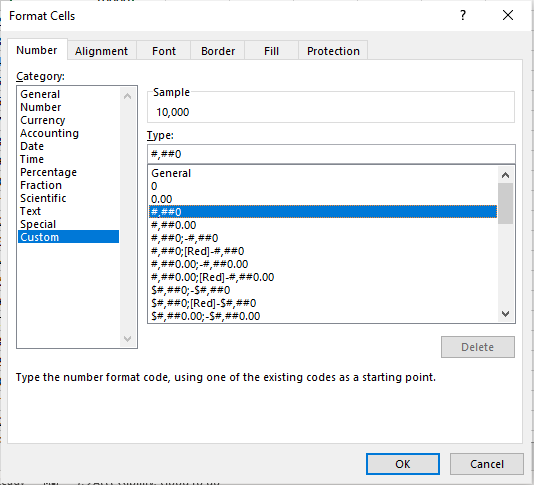
Step 4: In the Type field enter #,###, and click OK.
It is important to note when displaying the values in thousands that the value within the cell is still the same. This means that calculations can be conducted as normal and it will not affect a calculation.
3. Group The Columns
The third option is to group the columns. This option comes into play if you are in a situation where space on your display is at a premium and you have difficulty displaying all the columns that you want. As a result of this, it is necessary to try and squeeze in all information that you need into a screen which sometimes results in you getting the display ####.
What grouping in columns does is allow you to do is group a series of columns together and then hide them as required and display them again as necessary. To do this the following steps are required;
Step 1: Select the columns that you wish to group

Step 2: Select the data tab and then select group and group again which is located to the far left of the ribbon in Excel,

Step 3: Once these selections are made a negative button will appear above the column selected. Selecting the button will allow a series of columns to be hidden from view which will create additional space on the spreadsheet as required. This is a useful option for maximizing the availability of visible space on the screen reducing the need for the size of the columns to be reduced.

Relevant Articles
How Do You Copy A VLOOKUP Formula Without Changing The Table Array?
Why Is The Vlookup Returning #N/A When Value Exists? What Is The Problem And How To Fix It?