Can You Do An If Statement In Excel Based On Cell Formatting Such As Color? (It Is Possible Without VBA) -

One of the most common questions we get asked is is it possible to produce an if statement based on cell formatting such as the background color of a cell or whether it has borders, a particular type format or even the cell alignment.

It is possible to use an if statement to identify cells based upon formatting which can include a number of the aspects of the cell which include its color, the color of the text, the alignment of the text and many other characteristics. This can also be done without needing to be able to program in VBA.

However, to achieve this it requires you to create a get cells function within Excel with the correct characteristics to ensure that you can differentiate between cells with different formatting which is not terribly difficult.

How To Create A Get Cell Function

To create a get cells function is relatively straightforward and as mentioned above it can be modified to cover a range of cell formats but for the purposes of this article we will look at how to create a get cell function for color.

Step 1 – Go To The Formulas Tab and then select Name Manager

Step 2 – Click New To Create the Get Cell Function

Step 3 – Name the function you are creating. Note that it is best to give the function a name that makes sense and you can find later if necessary. Enter =Get.cell(38,Sheet1!A1) in the Refers to: area.

Notes: In the get cell command the first argument defines the type of cell formatting that you are looking for in the Formula. In this case 38 is the number that is required for the background color of a cell. There is a list of all the different arguments at the end of the article which will allow you to find exactly the formatting you need to identify in your formula.

Secondly. the default of Excel when you select a cell on your page is to reference the cell with dollar signs which is shown in the screenshot above. To make the cell reference copyable you need to remove the dollar signs from the formula.

Step 4 – Once you click ok on the previous screen you will get the name manager screen come up which you just need to click close to complete the creation of the get cell function.

How To Apply The Get Cell Function In An If Statement

Having created the get cell function for your desired formatting, in this case color, you can then use it in an if statement to create the function that will be able to pick out the cells with the correct format.

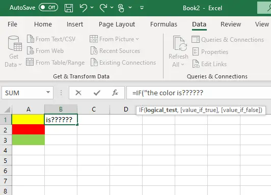
To do this enter the equals sign and select from your list of functions the name of the getcell function of created which in my example is cellcolor. In the screenshot below you will see that once you have created the function it will appear in the list of possible functions you can use with an Excel. Enter =cellcolour to enter it into the cell

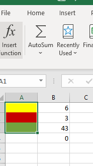
When you apply the cell formula to the different cells with different colors you will see that it produces a different number for each color in the cell including the number 0 in cases where there is no color formatting. This can then be used within an if statement to identify the color of the cell and therefore apply a logic statement around it.

However, it’s important to note that if you do not get the expected result then double check the cell references that you are using to ensure that you are in the correct columns. For example when I was setting up this example I used cell A1 as the reference. However, when I actually applied the cell color to the cells in B1 the cell reference became B1 and therefore did not return the expected result.

Finally, you will need to create a nested if statement depending upon the specific colors in the example that we want to identify. In this example I will create an if statement that returns true if any of the cells contain a colors which is as follows;

=if(cellcolor=0, “cell has no color”, “cell has color”)

Creating An If Statement For Other Types Of Formatting

Exactly the same method can be used to create an if statement for any type of formatting provided that you know the argument required for each one of the different formatting styles covered. A list of the relevant numbers for the cell argument are provided below for your reference.

Get Cell Argument	Description	Comment
1	Absolute reference of the upper-left cell in reference, as text in the current workspace reference style.
2	Row number of the top cell in reference.
3	Column number of the leftmost cell in reference.
4	Same as TYPE(reference).
5	Contents of reference.
6	Formula in reference, as text, in either A1 or R1C1 style depending on the workspace setting.
7	Number format of the cell, as text (for example, “m/d/yy” or “General”).
8	The cell’s horizontal alignment. Function returns 1 to 7 depending on the alignment.	1 = General, 2 = Left, 3 = Center, 4 = Right, 5 = Fill, 6 = Justify, 7 = Center across cells
9	The left-border style assigned to the cell: Function returns 1 to 7 depending on the alignment.	0 = No border, 1 = Thin line, 2 = Medium line,3 = Dashed line, 4 = Dotted line, 5 = Thick line, 6 = Double line, 7 = Hairline
10	The right-border style assigned to the cell. Function returns 1 to 7 depending on the alignment.	0 = No border, 1 = Thin line, 2 = Medium line,3 = Dashed line, 4 = Dotted line, 5 = Thick line, 6 = Double line, 7 = Hairline
11	The top-border style assigned to the cell. Function returns 1 to 7 depending on the alignment.	0 = No border, 1 = Thin line, 2 = Medium line,3 = Dashed line, 4 = Dotted line, 5 = Thick line, 6 = Double line, 7 = Hairline
12	The bottom-border style assigned to the cell. Function returns 1 to 7 depending on the alignment.	0 = No border, 1 = Thin line, 2 = Medium line,3 = Dashed line, 4 = Dotted line, 5 = Thick line, 6 = Double line, 7 = Hairline
13	Cell pattern for selected cell.	Returns a number from 0 to indicating the pattern of the selected cell. If no pattern is selected, returns 0.
14	The cell is locked	If locked TRUE; otherwise, returns FALSE.
15	The cell’s formula is hidden	If hidden TRUE; otherwise, returns FALSE.
16	A two-item horizontal array containing the width of the active cell and a logical value indicating whether the cell’s width is set to change as the standard width changes (TRUE)or is a custom width (FALSE).
17	Row height of cell, in points.
18	Name of font, as text.
19	Size of font, in points.
20	The text is bold	If all the characters in the cell, or only the first character, are bold, returns TRUE; otherwise, returns FALSE.
21	The text is Italic	If all the characters in the cell, or only the first character, are italic, returns TRUE; otherwise, returns FALSE.
22	The text is Underlined	If all the characters in the cell, or only the first character, are underlined returns TRUE; otherwise, returns FALSE.
23	The text is struck through	If all the characters in the cell, or only the first character, are struck through, returns TRUE; otherwise, returns FALSE.
24	Font Color	Font color of the first character in the cell, as a number in the range 1 to 56. If font color is automatic, returns 0.
25	The characters in the cell are outlined	If all the characters in the cell, or only the first character, are outlined, returns TRUE; otherwise, returns FALSE.Outline font format is not supported by Microsoft Excel for Windows.
26	Shadow Font	If all the characters in the cell, or only the first character, are shadowed, returns TRUE; otherwise, returns FALSE.Shadow font format is not supported by Microsoft Excel for Windows.
27	Page Break at the cell	0 = No break, 1 = Row, 2 = Column, 3 = Both row and column
28	Row level (outline).
29	Column level (outline).
30	If the row containing the active cell is a summary row, returns TRUE; otherwise, returns FALSE.
31	If the column containing the active cell is a summary column, returns TRUE; otherwise, returns FALSE.
32	Returns the name of the workbook and sheet	Name of the workbook and sheet containing the cell If the window contains only a single sheet that has the samename as the workbook without its extension, returns only the name of the book, in the form BOOK1.XLS. Otherwise, returns the name of the sheet in the form “[Book1]Sheet1”.
33	Formatted To Wrap text in cell	Returns true of false
34	Left-border color	Returns color as a number in the range 1 to 56. If color is automatic, returns 0.
35	Right-border color	Returns color as a number in the range 1 to 56. If color is automatic, returns 0.
36	Top-border color	Returns color as a number in the range 1 to 56. If color is automatic, returns 0.
37	Bottom-border color	Returns color as a number in the range 1 to 56. If color is automatic, returns 0.
38	Shade foreground color	Returns color as a number in the range 1 to 56. If color is automatic, returns 0.
39	Shade background color	Returns color as a number in the range 1 to 56. If color is automatic, returns 0.
40	Style of the cell, as text.
41	Returns the formula in the active cell without translating it (useful for international macro sheets).
42	The horizontal distance, measured in points, from the left edge of the active window to the left edge of the cell.	May be a negative number if the window is scrolled beyond the cell.
43	The vertical distance, measured in points, from the top edge of the active window to the top edge of the cell.	May be a negative number if the window is scrolled beyond the cell.
44	The horizontal distance, measured in points, from the left edge of the active window to the right edge of the cell.	May be a negative number if the window is scrolled beyond the cell.
45	The vertical distance, measured in points, from the top edge of the active window to the bottom edge of the cell.	May be a negative number if the window is scrolled beyond the cell.
46	Cell contains a text note	A text note, returns TRUE; otherwise, returns FALSE.
47	Cell contains a text note	A sound note, returns TRUE; otherwise, returns FALSE.
48	Cells contains a formula	A formula, returns TRUE; if a constant, returns FALSE.
49	If the cell is part of an array, returns TRUE; otherwise, returns FALSE.
50	The cell’s vertical alignment:	1 = Top, 2 = Center, 3 = Bottom, 4 = Justified
51	The cell’s vertical orientation.	0 = Horizontal, 1 = Vertical, 2 = Upward, 3 = Downward
52	The cell prefix (or text alignment) character, or empty text (“”) if the cell does not contain one.
53	Contents of the cell as it is currently displayed, as text, including any additional numbers or symbols resulting from the cell’s formatting.
54	Returns the name of the PivotTable view containing the active cell.
55	Returns the position of a cell within the PivotTableView.
56	Returns the name of the field containing the active cell reference if inside a PivotTable view.
57	Superscripts	Returns TRUE if all the characters in the cell, or only the first character, are formatted with a superscript font; otherwise, returns FALSE.
58	Font Style	Returns the font style as text of all the characters in the cell, or only the first character as displayed in the Font tab of the Format Cells dialog box: for example, “Bold Italic”.
59	Underline Style	1 = none, 2 = single, 3 = double, 4 = single accounting, 5 = double accounting
60	Subscript	Returns TRUE if all the characters in the cell, or only the first character, are formatted with a subscript font; otherwise, it returns FALSE.
61	Returns the name of the PivotTable item for the active cell, as text.
62	Name of workbook and sheet	Returns the name of the workbook and the current sheet in the form “[book1]sheet1”.
63	Returns the fill (background) color of the cell.
64	Returns the pattern (foreground) color of the cell.
65	Returns TRUE if the Add Indent alignment option is on (Far East versions of Microsoft Excel only); otherwise, it returns FALSE.
66	Name of workbook	Returns the book name of the workbook containing the cell in the form BOOK1.XLS.