Why Is My VLOOKUP Returning Wrong Value? How To Fix The Problem -

Have you ever had the experience of using a VLOOKUP, which is usually so reliable and then getting the function returning a value that you know just is not right. What is the reason for this and how can I fix the problem?

A VLOOKUP can produce unexpected results for a couple of different reasons which are listed below;

The VLOOKUP is set to produce an approximate match rather than an exact match.

There is more than one lookup value within your table array. In this case it will return the first value that it finds.
You have not fixed the position of the table array in the formula and it has changed when the formula was copied to another cell.
The wrong column reference has been selected.

The lookup value is present in the table array with different case settings on the letter giving you an unexpected result (this is extremely rare)

The VLOOKUP Is Set To An Approximate Match

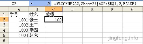
The Syntax for the vlookup with an Excel is as follows;

VLOOKUP (lookup_value, table_array, col_index_num, [range_lookup])

where;

Lookup_value is the value that you are trying to find in the table array.

Table_array is the area in the spreadsheet where you are looking for the lookup value.

Col_index_num designates which column the value should come from. The first column within the Table array equals 1, the second column within the table array equals 2…etc.

Range_lookup Argument within the function designates whether an exact or approximate match is being sought. True equals an approximate match, false equals an exact match.

The VLOOKUP can be set to an approximate match either by entering the value “TRUE” into the last argument within the VLOOKUP or alternatively not entering an argument at all.

The range lookup argument is optional within this particular function which Excel designates by placing square brackets around that function. In this particular function the default value if not entered is true which gives you an approximate match. If either of these events occur there is a possibility that the VLOOKUP will not return the value that you were expecting.

There Is More Than One Lookup Value In The Table Array

The other likely cause of an unexpected value in a VLOOKUP is in cases where there are multiple values in the table array that match the lookup value. This sort of event often occurs in things like sales reports where the same product may appear multiple times being purchased by different customers.

If you are looking for the sales value in these circumstances what will happened is that the VLOOKUP will return the first value that it finds in the table array which means that you may not be getting the value that you were expecting.

To overcome this issue the easiest way to deal with it is to use data tags from more than one cell to ensure that you have a unique look up value within your table array. In the example above you would need to have a lookup value that combined both the customer name and the product name to create our unique lookup value.

To do this it will be necessary to create a new column at the start of the table array which combines this data. This can be done relatively easily by using the CONCATENATE function or alternatively using an end between the cell references.

Examples

=Concatenate(A1, A2) OR =A1 & A2

To match the values in the table array you will also need to combine the Salvation in the vlookup formula an example of how to do this is shown below;

=vlookup(A1 & A2, B:D, 2, FALSE)

=vlookup(Concatenate(A1, A2), B:D, 2, FALSE)

The Position Of The Array Is Not Fixed

The other issue that can occur with a VLOOKUP which can create an unexpected result is cases where the formula has not been incorrectly set up to enable it to be pasted to different cells. This problem is more likely to occur in cases where the array reference refers to specific cells rather than entire columns.

In this circumstance what can happen is the range of table array can move downward if the formula is copied down a column for example. This can result in the VLOOKUP missing the first time that a lookup value appears in the table array..

This can be overcome fairly easily by using dollar signs in front of the cell references for the array which will stop the problem. The shortcut for putting the dollar signs into a formula is the F4 which will toggle through all the different dollar signs settings if you click on the cell reference in the formula. An example of dollar signs being used in the formula is provided below;

=vlookup(Concatenate(A1, A2), B:D, 2, FALSE)

The Wrong Column Reference Has Been Selected

Selecting an incorrect column reference will also cause you to produce an unexpected result. This typically happens when the array does not start in column A or people miscount. This can be quickly remedied by simply double-checking that you have the correct cell reference by recounting the columns to ensure it produces the result that you expect.

Case Setting Of The Lookup Value Are Different

VLOOKUP is a case insensitive function like most of the ones used in Excel with a couple of exceptions. The fact that it is case insensitive can sometimes cause an unexpected result to occur. This primarily occurs because the differences in case settings of the text can cause the cells to appear to look different even though Excel recognises them as being exact matches.

Generally, this problem is rare and can be overcome by using the INDEX MATCH method which will produce a case-sensitive result and works in the same way as a VLOOKUP. This particular method is case-sensitive because the MATCH function is case sensitive.

To show the syntax of INDEX MATCH we have provided the structure of a VLOOKUP and an INDEX MATCH function that will produce exactly the same result below.

=vlookup(A1), B:D, 2, FALSE)

=INDEX(B:D,MATCH(A1,B:D,0),2)