How To Get Trendline Equation In Excel (2 Methods: In A Cell Or In A Graph) -

How to get the trendline equation in an excel graph can sometimes be challenging to get, however, in this article we will cover two methods that will allow you to get the trendline equation or line of best fit for some linear data.

All lines can be described using the general linear equation listed below;

y = mx + c

where;

m = the gradient or slope of the line, and

c = the y-intercept which is the value of why at the point at which the line crosses the y-axis

Method 1 – Calculating The Equation In A Cell

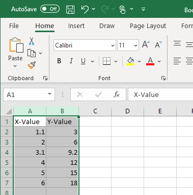
The first methods listed in this article will provide an Excel equation that will automatically produce the equation of the line of best fit or trendline in excel provided that the X values are placed in column A of the sheet and the Y values are placed in column B. The equation required to do this is as follows;

=”Y = ” & ROUND(SLOPE(B:B,A:A), 2) & IF(INTERCEPT(B:B,A:A)<0, “x “, “x + “) & ROUND(INTERCEPT(B:B,A:A), 2)

Explanation Of The Formula

Slope Function: Provides the slope or gradient of the line of best fit and its structure is Slope(Y values, X Values). In the example above I have opted to select the entire column in both cases because that means that the formula does not need to be adjusted even if additional data is added.

Intercept Function: Provides the y-intercept for the equation and has the same structure as slope.

Round Function: Rounds results of the slope and intercept functions 2 two decimal places in this example because otherwise, the formula produces a large number of decimal places. the number of decimal places required can be easily adjusted by adjusting the number it’s in the round function. ie the number in bold could be adjusted: ROUND(INTERCEPT(B:B,A:A), 2)

If Function: The function is necessary within the formula to.allow.for both positive and negative intercepts within the formula. As a result the logic test within the if statement checks whether the gradient is less than 0 which avoids the situation where you have a positive sign and a negative sign sitting next to each other if the gradient is negative.

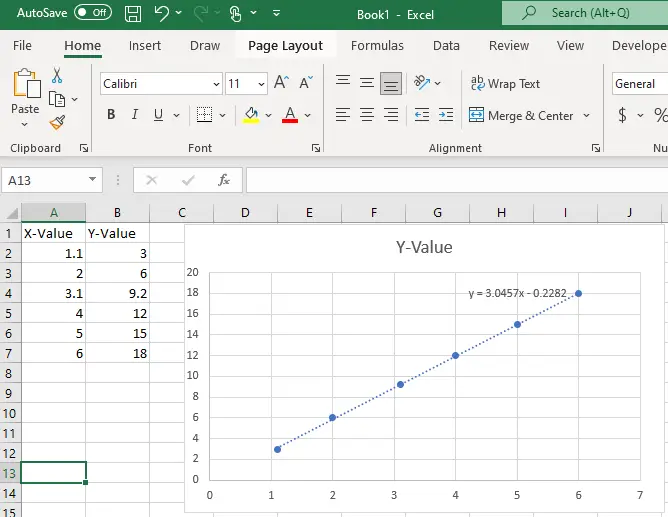
Method 2: Getting The Trendline Equation From A Graph

The second method listed more commonly used by excel users is graphing the data and getting the graph to show the equation of the trendline. The disadvantage of this method is that if the values in the equation are required for additional calculations they need to be manually inserted into a spreadsheet.

Whereas the formulas above can be adjusted to extract the slope and intercept allowing calculations to be done without the need to graph the data.

How To Get The Trendline From The Graph

Step 1: Highlight the data to be graphed

Step 2: Select insert on excel’s ribbon and then select the scatter graph

Step 3: Once the graph appears then right click on one of the data points and select ‘Add Trendline.

Step 4: A panel titled Format Trendline will appear on the right handside of the screen. Scroll down to the bottom and select the Display Equation on the chart. It should appear on the chart