What $ Does In Excel Formulas? How To Use Them And Handy Shortcuts -

If you are using Excel regularly but not an experienced user you may come across formulas that have dollar signs in them and you may be wondering what they actually do in the formulas and why are people put them in.

$ signs are added to the formula to control what happens to cell references when the formulas are copied to another location within a spreadsheet. The default setting within Excel is that cell references will change when the Formula is copied to another location.

Example

Cell A1 contains the formula =B1+C1. When the formula is copied down to A2 the formula will automatically be adjusted to =B2+C2.

This default setting in Excel is beneficial in many cases because it allows you to quickly copy formulas into the cells and have Excel automatically adjust them for you. In the example above if you have two columns of numbers that need to be added together in columns B and C the default setting is quite convenient.

However, there are certain circumstances where the default setting does not work well and that is where $ signs come in. The $ signs can be used to fix the position of the cell reference references when copying a formula.

The dollar signs can be applied to cell references in 3 different ways depending upon what is required these three conditions are as follows;

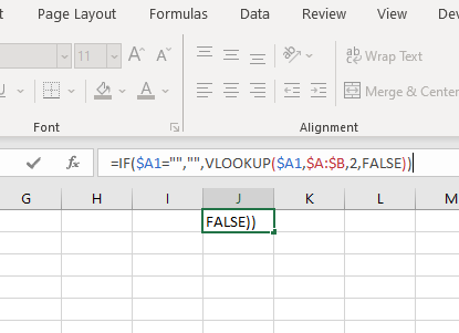
Fixing The Column Reference: =$A1

Fixing The Row Reference: =A$1

Fixing Both The Column And Row Reference: =$A$1

The dollar sign fixes the position of the cell reference element that it is in front of. In cases where you are only referencing the column, ie B:B, a dollar sign in front of the column letter will fix the position of the column.

In cases where there is a range being designated, ie A4:B52, if you need to fix the entire range you need to place dollar signs in front of both cell references. ie $A$4:$B$52.

Useful Shortcuts That Will Save You Time

There are several shortcuts within Excel that will speed up the process of adding dollar signs and also redistributing your formula around your spreadsheet.

Tip 1: Applying $ Signs To Formula

There is a shortcut with Excel that will allow the dollar signs to be applied to cell references quickly and easily. To do this start by clicking on the cell reference that you wish to apply the dollar signs to. Hit their F4 key repeatedly to toggle through the four possible dollar sign settings for cell reference;

no $ signs,
$ sign in front of the Columns
$ sign in front of the Row

$ signs in front of both

Tip 2: Copying Formulas Down A Column Instantly

This shortcut is useful in cases where you need to copy formulas down a column and you have large amounts of data that extends down the page by several thousand lines. To apply the shortcut, create the formula that you want at the top of the column. In the example below I have created a Formula in Cell C1.

To copy that formula down the column, place your mouse above the little square in the bottom right-hand corner of the cell containing the formula, in the example below this would be cell C1. To see the cursor change to a plus sign double click.

Once you double-click on the square the formula will be automatically copied all the way down to the last line of data which can save a lot of time. However, it is important to note that the formula will not extend all the way down the full length of the data if there is a gap in the data, ie lines are missing.

The other reason that copying the formula will not extend the full length of the data is if there is information already in cells further down in the data. In these circumstances what will happen is that the formula is copied down until it reaches a cell that is occupied with data.

Tip 3: Prepare Multiple Formulas In Cells

The third tip that we recommend that you follow is useful in cases where you have to apply several formulas.to a piece of data. An example of this might be when you are below vlookup in multiple columns from a separate piece of data.

In this circumstance it is most efficient to prepare the formulas is to prepare the first formula with dollar signs to fix the lookup value as well as the table array. An example of this is provided below;

=vlookup($A2, $AA$2:$ZZ$1000, 5, FALSE)

Note: The lookup value has only the column reference fixed because you will need to copy it down.

This will allow the formula to be copied across columns and modified to suit the particular data that you want to call up using the vlookup function. All that is required is to change the column number to the relevant reference.

Once the formulas have been prepared in the top row they can all be highlighted and tip 2 can be applied to the formulas by double-clicking on the square in the bottom right-hand corner of the group of cells which will result in all formulas being copied down the columns.